Big O
Asymptotic analysis is defining the mathematical framing of an algorithm run-time performance. This helps us in concluding the best case (minimum time required to run execution), average case and worse case (maximum time required for run execution) scenario of an algorithm. For example, f(n) means it increases linearly, for g(n^2) it increases exponentially. Asymptotic Notations are O-notation, Omega-notation and Theta Notation.
Big O Notation: Formal way to express the upper bound of an algorithm’s running time. It measures the worse case time complexity of the longest amount of time an algorithm can possibly take to complete.
Omega Notation: is the formal way to measure the lower bound of an algorithm running time. It measures the best time to complete an algorithm
Theta Notation: It expresses the lower and upper bound of an algorithm running time.
| Common Asymptotic Notations | Term | Definition | Example |
|---|---|---|---|
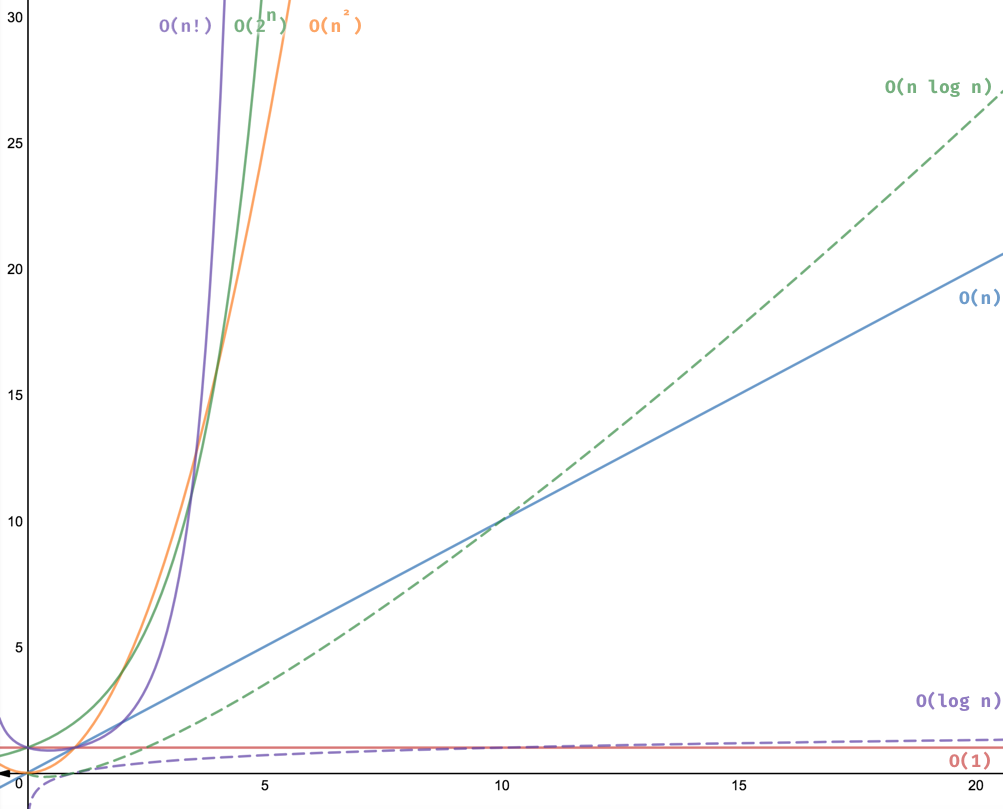
| Constant | O(1) | Program will run the same length regardless of input size | Stack push, pop and peek, Queue, enqueue and dequeue, insert a node into a linked list |
| Logarithmic | O(log n) | The time taken is proportional to the logarithm of the amount of data. The impact of increasing data on time lessens as the data grows | Binary search a sorted list, search a binary tree, merge sort, heap sort, quick sort |
| Linear | O(n) | Program will run proportionally to the size of the input | Linear Search, count items in a list, compare a pair of strings |
| Linearithmic | O(n log n) | The time taken is proportional to the logarithm of the amount of data multiplied by the amount of data | Merge sort and Quick sort |
| Quadratic | O(n^2) | Doubling the size of the input will quadruple the running time | Bubble sort, selection sort, insertion sort, traverse a 2D array |
| Cubic | O(n^3) | Doubling the size of the input will have a cubic effect on the running time | - |
| Polynomial | O(n^k) | Time taken is proportional to the amount of data raised to the power of a constant. If K is 2 then is quadratic, if k is 3 then it is cubic complexity. K can be any number | one can think of constant, linear, quadratic and cubic are examples of polynomial. |
| Exponential | O(K^n) | Time taken is proportional to a constant raised to the power of the amount of data | n-Queen problem, Travelling salesman, password cracking that operates by brute force |
| Factorial | O(n!) | Doubling the size of the input, will have a factorial effect on the time |
To summarize, the concept of asymptotic complexity is to draw an equivalence between functions as their input approaches infinity.
How to calculate the asymptotic time complexity of the above algorithms?
Generally, by calculating how many times a statement will execute when the data doubles. WE calculate the rate of growth of time in respect to the input size.
Understanding Big O in plain english
There can be several ways to implement a for-loop or an if-statement when programming in python. There are also several ways in which these algorithms can be designed to interact with each other. But how do we measure the performance of these different implementations ? This is where we consider the time complexity and space complexity of the algorithms implemented. In case of time complexity, this will specifically measure the impact of more data vs the time it needs to execute the function. In case of space complexity, this will measure the impact of more data vs the amount of memory required to execute the function. The goal of any algorithmic design is to have the shortest time and take the least amount of space as possible.
Time Complexity
Time complexity quantifies the amount of time it takes by the algorithm to run as a function of its input length, n. The order of growth is the correlation between time and length of the input. If the length increases by x amount, how much more time does it take ?
The time complexity of an algorithm can be expressed using the following asymptotic notations.
O-notation: (pronounced “big-oh of g of n”): Denotes the asymptotic upper bound (An asymptotic line is a line that gets closer and closer to a curve as the distance gets closer to infinity.) for a given function.
\Omega()-notation: (pronounced “big-omega of g of n”): Denote the asymptotic lower bound for a given function.
\Theta()-notation:(pronounced “big-theta of g of n”): Denotes the asymptotic tight bound for a given function.
When considering time complexity, we look at the O-notation since it gives as the upper limit of execution. Generally, Big O Notation is the language we use to describe the complexity of an algorithm. Big O notation talks about how quickly the runtime grows in relative to the input. For instance, “runtime grows on the order of the size of the input O(n)” or “on the order of the square of the size of the input (O(N^2))”
Space Complexity
Space complexity quantifies the amount of memory the algorithm needs to execute as a function of its input length, n. Space complexity includes both auxiliary space and space used by the input. Space complexity is commonly expressed using the Big O notation. When we talk about space complexity we talk about the additional space taken and not the space already taken by the input. Space complexity is increased by variables, data structurs, function calls and allocations.
The auxiliary space is the temporary space the algorithm needs while getting executed.
How to measure Big O
To measure Big O, we go through each line of code and ask the question, how many times a line is getting executed in relatation to the input size ?
For example a “for-loop and if” is O(n) since it loops through each line of code and checks every input. While a “for loop - for loop” is O(n^2), since the number of loops are quadratic in relation to the input.
Rule 1: Worse Case - We calculate the worse case to represent our algorithm. Rule 2: Remove Constants - When having 1+O(n), or O(3n), then we drop the constant values, so it will be O(n) Rule 3: Different Terms for Inputs - this is a tricky one, if you have a function with 2 inputs for example
def run(value1, value2):
    for x in value1:
        print(x)

    for y in value1:
        print(y)
The Big O of this will be actually O(a+b) and not O(n). Since there is no gurantee what the value of Value 2 and Value 1 are. Value 1 can be 1million while Value 2 can be 4, so we represent this as O(a+b).
Rule 4: Drop Non-Dominant Values - If you have two for loops, or slower
Check https://www.bigocheatsheet.com/ for more graphs on different data structures.
Examples of Big O:
Imagine we have 10 items and a target value that take certain amount of memory when the algorithm is running. Worse case, if we double our items to 20 items, then it will take double the time to execute the function. This means that the time taken is proportional to the amount of data. This is known as “Linear Time Complexity” - O(n). The amount of memory required does not change since we still hold one target value in the memory. Therefore, the amount of memory required stays constant regardless of the amount of data. Therefore, the linear search has a constant space complexity O(1). Other examples that have constant space complexity are the bubble sort, insertion sort and the selection sort.
For the Quick Sort: Quick sort is a divide and conquer algorithm which creates two empty arrays to hold elements less than the pivot value and elements greater than the pivot value, and then recursively sort the sub arrays. There are two basic functions, swapping items in place and partitioning a section of the array.
In worse case scenario, if you want to sort a list of 8 items, you need (7 + 6 + 5 + 4 + 3 + 2 + 1) which is a total of 28 comparisons for 8 items. What if we double the list to 16 ? then it will (15+14+…..) which is a total of 120. The relation between the amount of data and the amount of processing required is not linear, since when we double the input data, the number of processes increase. The time complexity is quadratic. O(n^2) (O - n squared) since if we double the amount of input data, the processing roughly quadruples. For space complexity, if we double the amount of data, we need the double amount of stacks to hold the data. Therefore, Quicksort has a linear space complexity O(n) since quicksort relies on recursive calls.
Amortized Time:
Amortized is an interesting concept. Let us think of a dynamic array which expands as you add components. For example, an empty array with 100 slots, everytime you had an element, it will take up to one space. Therefore the time complexity is said to be O(1), up until when you hit the 100th slot, the dynamic array increases the size in double, to 200. In this case, the time complexity is O(N), since we have to create a new array and copy all the elements over. So yes, although we have O(1) on every insertion of element, ones in a time, we get an O(N). This is captured by “Amortized Time”. In any case, as the dynamic array doubles, the number of times it needs to double decreases with time. For example, the size goes as follows, 100 -> 200 -> 400 -> 800 ….. The sum of all of these gives O(2X), dropping the contants, the amortized time is O(1) for each insertion.
Difference between best/worse/expected case and big O/theta/omega:
Best, worst and expected cases describe the Big time for particular inputs Big O, big omega and big theta desribes the upper, lower and tight bounds for the runtime
Summarize:
- Big O time complexity: Describes the impact of increasing the input data on the time taken for a program to running
- Big O space complexity: Describes the impact of increasing the input data on the extra memory needed by the program.
- Recursive algorithms require additional stack space for their processes.
Common way to talk about Big O notation:
- The function runs in O(1) meaning it has constant time in relative to its input
- The function runs in O(n) means in linear time where n is the number of items in the arrays
- The function runs in O(n^2) means it runs in quadratic time. For eg, nested for loops.
- Big O usually talks about the worse case scenario. But it is import to imply it when talking about Big O notation.
- Usually when we talk about space complexity, we’re talking about additional space, so we don’t include space taken up by the inputs